The post Kinetica’s Memory-First Approach to Tiered Storage: Maximizing Speed and Efficiency appeared first on Kinetica - The Real-Time Database.
]]>In an ideal scenario, all operational data would reside in memory, eliminating the need to read from or write to slower hard disks. Unfortunately, system memory (RAM) is substantially more expensive than disk storage, making it impractical to store all data in-memory, especially for large datasets.
So, how do we get the best performance out of this limited resource? The answer is simple: use a database that optimizes its memory use intelligently.
Prioritizing Hot and Warm Data
Kinetica takes a memory-first approach by utilizing a tiered storage strategy that prioritizes high-speed VRAM (the memory co-located with GPUs) and RAM for the data that is most frequently accessed, often referred to as “hot” and “warm” data. This approach significantly reduces the chances of needing to pull data from slower disk storage for operations, enhancing the overall system performance.

The core of Kinetica’s tiered storage strategy lies in its flexible resource management. Users can define tier strategies that determine how data is prioritized across different storage layers. The database assigns eviction priorities for each data object, and when space utilization in a particular tier crosses a designated threshold (the high water mark), Kinetica initiates an eviction process. Less critical data is pushed to lower, disk-based tiers until space utilization falls to an acceptable level (the low water mark).
This movement of data—where less frequently used information is shifted to disk while keeping the most critical data in high-speed memory—ensures that Kinetica can always allocate sufficient RAM and VRAM for current high-priority workloads. By minimizing data retrieval from slower hard disks, Kinetica can sidestep the performance bottlenecks that typically plague database systems.
The Speed Advantage: Memory vs. Disk
The performance gains achieved by this approach are clear when you consider the speed differential between memory and disk storage. To put things into perspective, reading 64 bits from a hard disk can take up to 10 million nanoseconds (0.01 seconds). In contrast, fetching the same data from RAM takes about 100 nanoseconds—making RAM access 100,000 times faster.

The reason for this stark difference lies in the nature of how data is accessed on these storage devices. Hard disks use mechanical parts to read data, relying on a moving head that accesses data in blocks of 4 kilobytes each. This block-based, mechanical retrieval method is inherently slower and incurs a delay every time data needs to be accessed. On the other hand, system memory allows direct access to each byte, without relying on mechanical parts, enabling consistent and rapid read/write operations.

Kinetica’s memory-first strategy leverages this inherent speed advantage by prioritizing RAM and VRAM for all “hot” data. This not only reduces the reliance on slower storage but also ensures that analytical operations can be performed without the bottleneck of data loading from disk.
Managing Costs Without Sacrificing Performance
While memory offers significant speed advantages, the flip side is its cost. Storing all data in RAM is prohibitively expensive for most organizations, especially when dealing with terabytes or petabytes of data. Kinetica balances this cost with two key approaches:
1. Intelligent Tiering: As mentioned earlier, Kinetica’s tiered storage automatically manages what data should stay in high-speed memory and what should be moved to lower-cost disk storage. This ensures that only the most crucial data occupies valuable memory resources at any given time.
2. Columnar Data Storage: Kinetica also employs a columnar data storage approach, which enhances compression and enables more efficient memory usage. By storing data in columns rather than rows, Kinetica can better optimize its memory footprint, allowing more data to be held in RAM without exceeding cost limits.
Conclusion
By adopting a memory-first, tiered storage approach, Kinetica effectively addresses the inherent challenges of traditional database systems. Its ability to prioritize RAM and VRAM for the most frequently accessed data—while intelligently managing less critical data on lower-cost disk storage—allows for faster analytics without the performance penalty of constant disk access.
This approach ensures that Kinetica remains an efficient, high-performance database solution, capable of handling complex analytics at speed, without requiring prohibitively large memory investments. In essence, Kinetica provides the best of both worlds: the blazing speed of memory with the cost efficiency of tiered storage management.
The post Kinetica’s Memory-First Approach to Tiered Storage: Maximizing Speed and Efficiency appeared first on Kinetica - The Real-Time Database.
]]>The post How to deploy natural language to SQL on your own data – in just one hour with Kinetica SQL-GPT appeared first on Kinetica - The Real-Time Database.
]]>You’re about to see how Kinetica SQL-GPT enables you to have a conversation with your own data. Not ours, but yours. With the built-in SQL-GPT demos, the data is already imported, and the contexts that help make that data more associative with natural language, already entered. When your goal is to make your own data as responsive as the data in our SQL-GPT demos, there are steps you need to take first.
This page shows you how to do the following:
- Import your data
Load their contents into tables inside Kinetica - Create contexts
These will provide the large language model (LLM) with the semantic information it needs to be able to reference the proper columns and fields in your tables - Ask Questions
Questions are phrased the way you’d say these questions out loud, then run the generated queries on Kinetica to get instantaneous results
STEP 1: Import your Data into Kinetica
Kinetica recognizes data files stored in the following formats: delimited text files (CSV, TSV), Apache Parquet, shapefiles, JSON, and GeoJSON [Details]. For Kinetica to ingest this data from another database or from a spreadsheet, it should first be exported from that source into one of these formats.
With one or more importable data files at the ready, here’s what you do:
- Log into Kinetica Workbench. If you don’t already have Kinetica setup, you can Create a Kinetica Cloud Account Free:
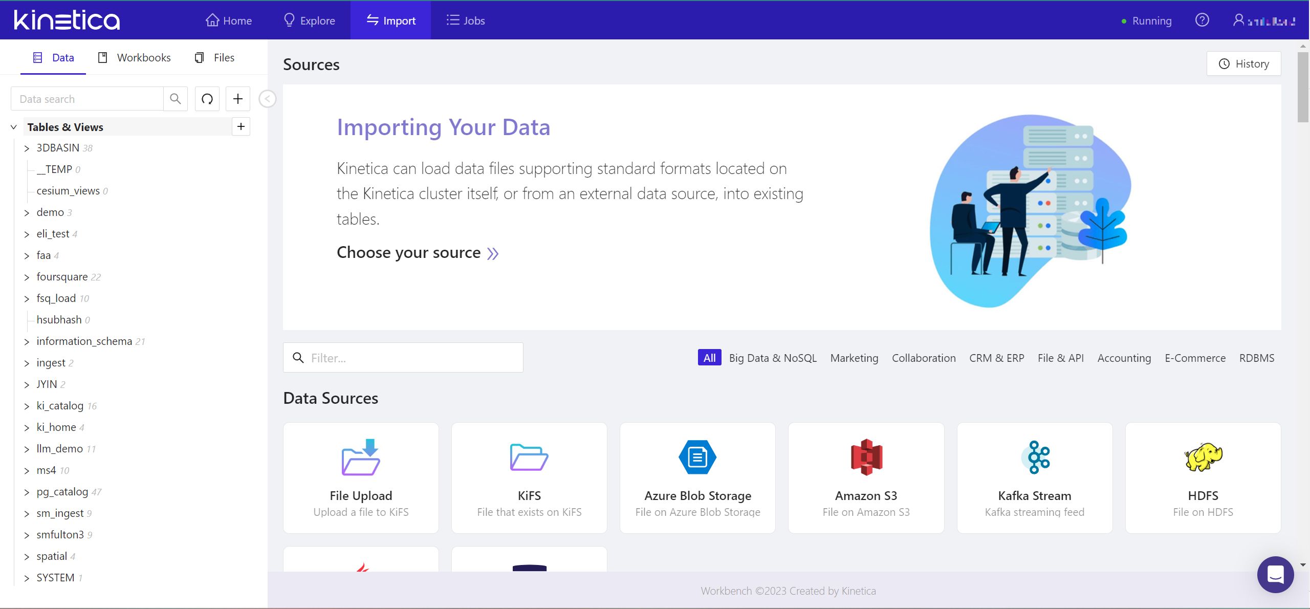
- From the menu over the left-side pane, click the Files tab. Hover over the + button, and from the popup, select Add New Folder.
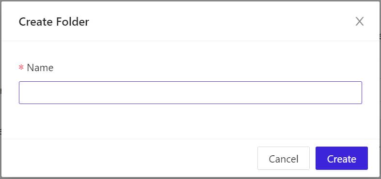
- In the popup window, under Name, enter a unique name, then click Create. The name you entered will soon appear in the Folders list in the left-side pane, sorted in alphabetical order and preceded by a tilde (~).
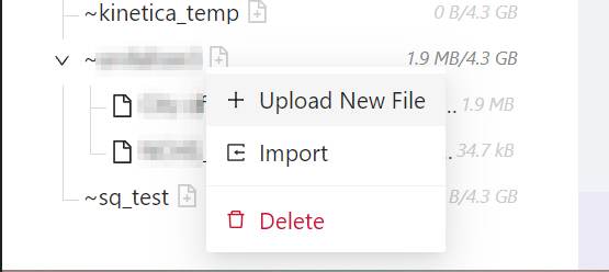
- In the Folders list, locate and right-click the name of your new folder. From the popup menu, select Upload New File. The Upload File panel will appear.
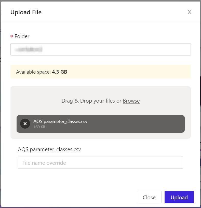
- From your computer’s file system, choose the file or files you wish to upload into your new Kinetica folder, so that their data may be imported. The files you chose will be indicated in the grey box in the center of the Upload File panel.
- Click Upload. Your data files will be uploaded into Kinetica, and this panel will keep you apprised of their progress.
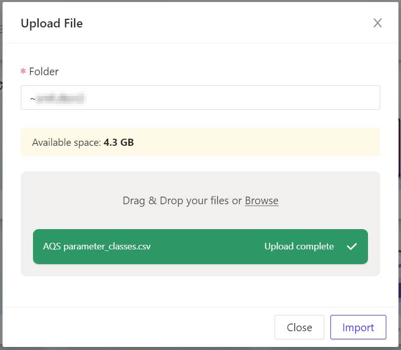
- In a moment, all the grey progress report bars will turn green, indicating your files are successfully uploaded. To proceed, click Import. The Kinetica Filesystem Import panel will appear.
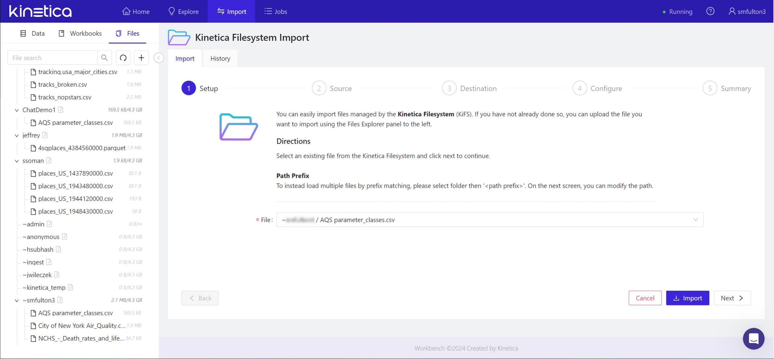
- In the panel marked 1 Setup, the file or files you’ve chosen for import will already have been entered. Click Next > to continue.
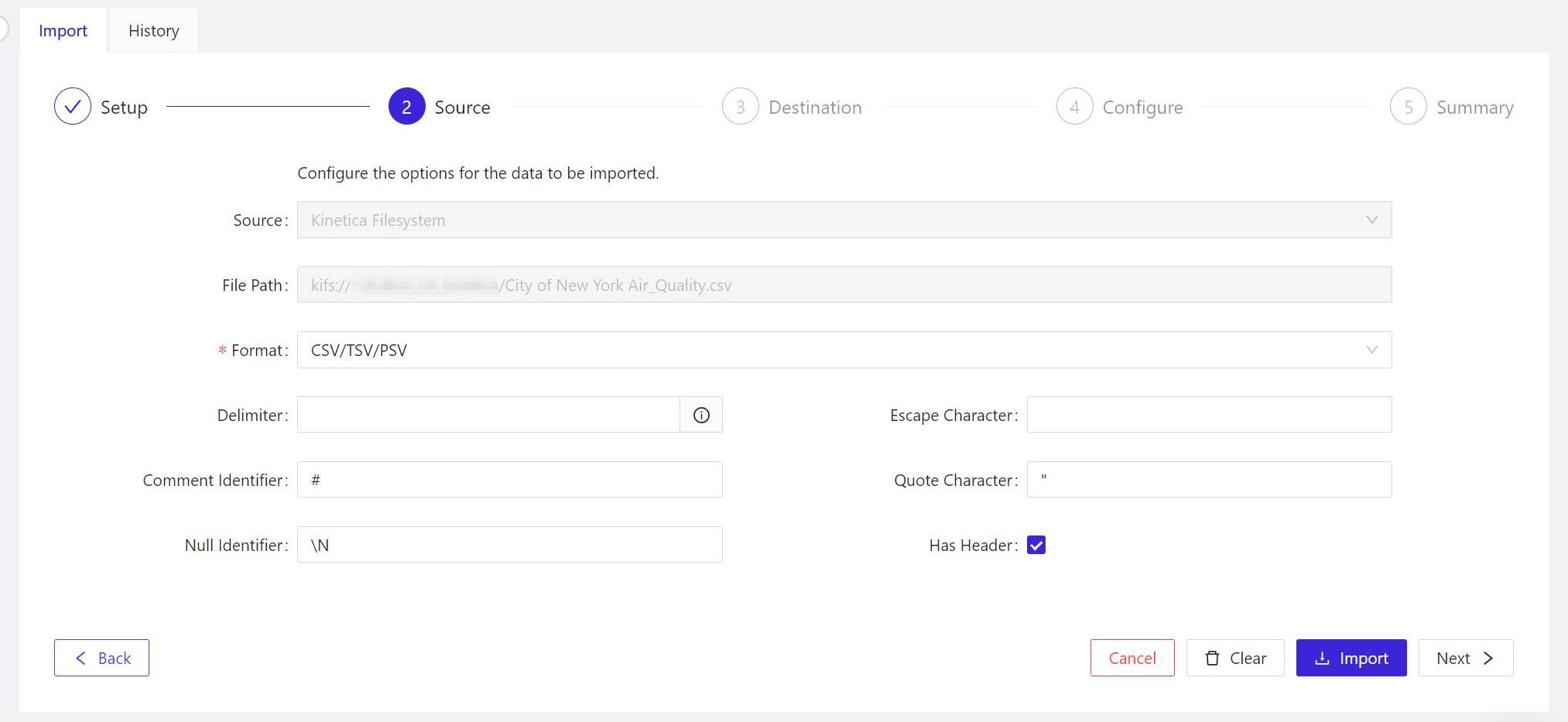
- For the panel marked 2 Source, Kinetica will have inferred which format your data is in already. If the event it makes an inaccurate assumption, in the Format field, choose the format for your imported data from the list. When all the options for this panel look correct, click Next > to continue.
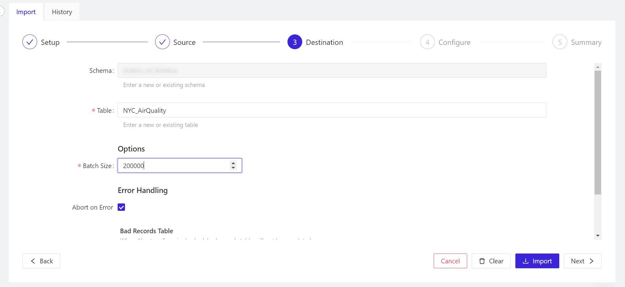
- In the panel marked 3 Destination, if you’re operating on the free tier, your edition of Kinetica will only have one schema, whose name will appear in the Schema field. By default, the name to be applied to the table is the current name of the data file (if you changed that name in step 4, your chosen name will appear here). When the options here are set, click Next > to continue.
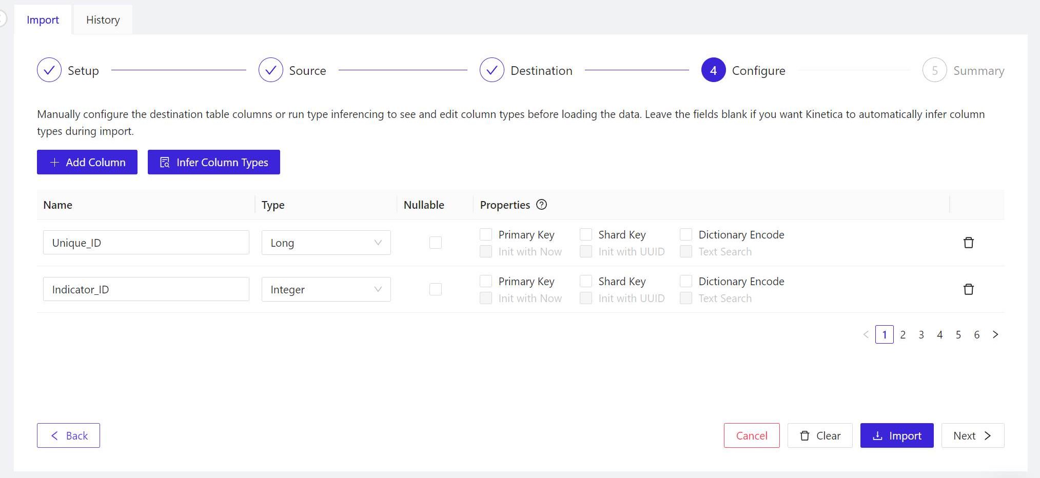
- For the panel marked 4 Configure, Workbench is usually capable of inferring the proper field names and content types (for example, short integer values versus floating-point values) from properly formatted, existing tables. So you may skip the manual inference step, and click Next > to continue.
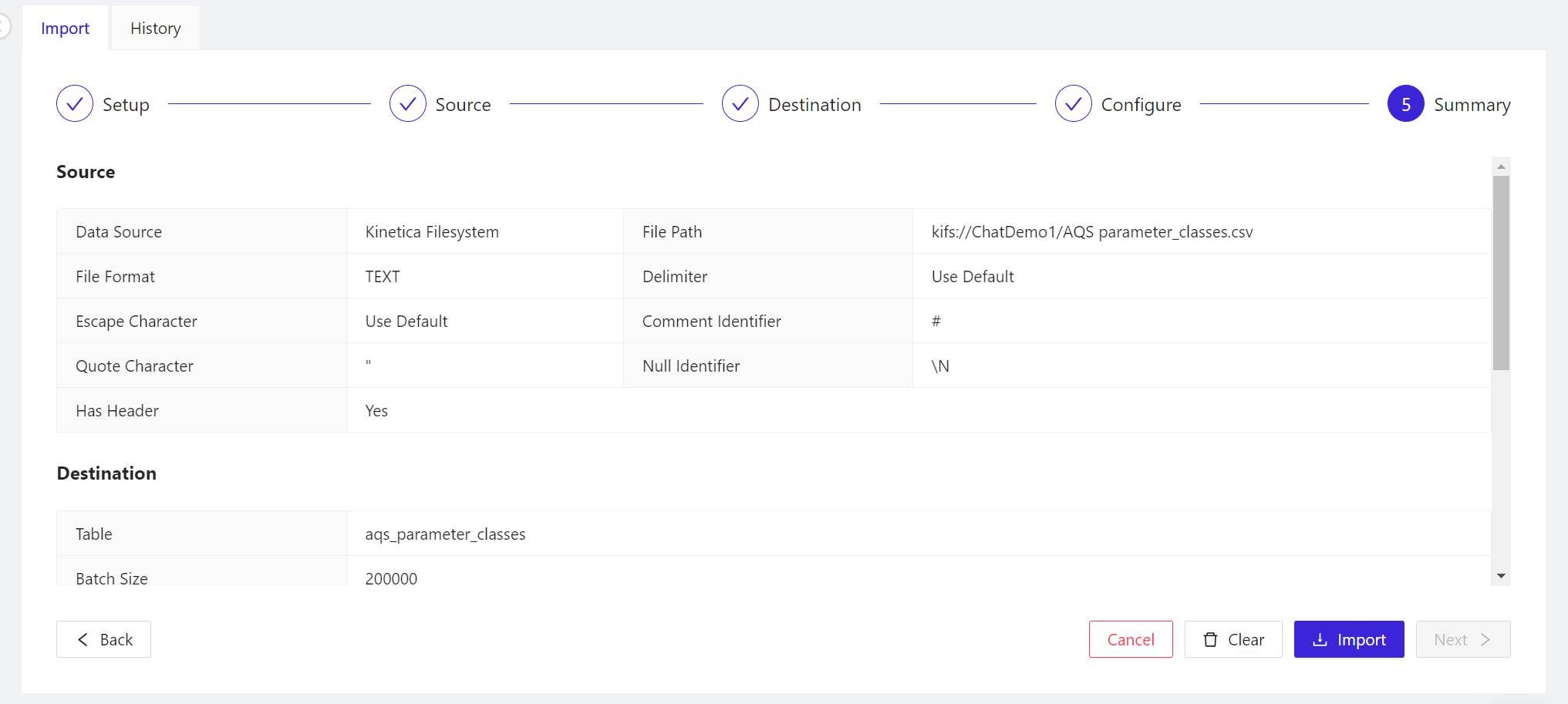
- The 5 Summary panel explains in detail what Kinetica is about to do with the data you’re asking Workbench to import. First, it reviews the options you’ve chosen. Scroll down to find the CREATE TABLE statement that Kinetica will use to generate the table for the schema, followed by the LOAD DATA INTO statement that will populate the new table with data from the file. There’s nothing more to import here, so when you’re ready to start importing, click Import.
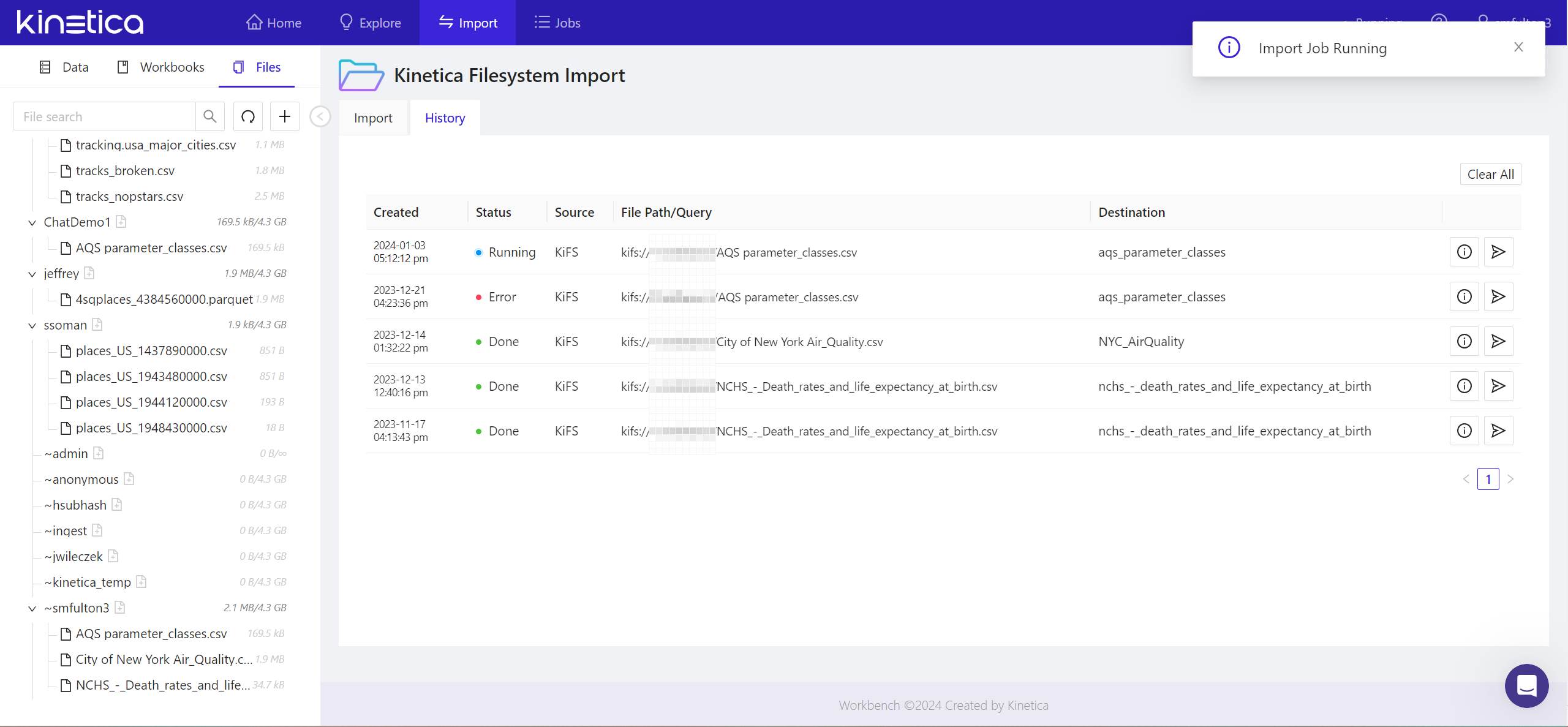
- The status of the import job will be tracked in the History tab. Once complete, you’ll see a notification to that effect in the upper right of the panel.
Your imported files should now be accounted for in the Files tab of the Workbench’s left-side pane. Look under your login name to locate them. The tables generated from that imported data should now appear in the Data tab of this same pane, in the subcategory Tables & Views, under the name of your schema.
STEP 2: Create Contexts for Imported Tables
With OpenAI’s ChatGPT, you’ve probably experienced the feeling of getting a sub-par response from what you thought was an articulate question. Language models can’t always infer the information you may have thought was obviously implied, if not explicitly asserted.
For SQL-GPT, you increase the probability of correlation between the generated SQL statements and the data you’ve just imported, by means of contexts. It’s a tool designed to give the language model the best possible information on the first go.
A context consists of natural-language explanations of the terms relevant to your data, for the benefit of the language model. In Kinetica, a context is a native database object that is created using the SQL statement CREATE CONTEXT. Workbench enables you to develop a comprehensive context with the annotations and associations it needs to connect ideas from a natural-language question, with terms in your database.
There are four components of a complete context:
- Table definition The set of table definitions in a context indicate what tables should be considered when generating SQL responses. The DDL for these tables including the column definitions are sent to the LLM during inferencing. Tables with many columns can quickly consume LLM context space and this should be limited to only what is necessary. You can optionally provide the LLM with a description for the table which is uUsually a single sentence or a brief note explaining what the data represents in its entirety. For example, “The median annual death rates per capita for United States citizens.”
- Rules – One or more instructions for the LLM regarding how to process or interpret data. For example, for geospatial data used in a Kinetica demo that includes the maps of the states, a rule may contain this instruction to apply a specific parameter: “Join this table using KI.FN.STXY_WITHIN()=1” The language model is capable of interpreting the sentence appropriately. Another example would advise the LLM to associate a field name airport_code with a phrase used to describe airports, such as “airport code” (without the underscore character) — as in, “Use airport_code to find the routing code for the airport.”
- Column descriptions – Instructions helping the language model to interpret the meanings of field names, giving it clues for associating their symbols (which may have no language definition at all) with everyday terms and phrases that people generally use, coupled with terms that are specific to the data set For example, in a data set that includes the perimeter points, or “fences,” for given areas on a map, a good context may include a column named WKT. It’s not obvious to a language model what that means, or that it’s a common abbreviation for the geospatial abbreviation for Well-Known Text format. So a good column description might include, “A well-known text description of the spatial outline or perimeter of each fence.”
- Samples – An appropriate sample would include an example of a natural-language question you would expect yourself or another user to ask, coupled with an actual Kinetica SQL statement you’ve tried successfully in Kinetica. Samples should reference only the names of tables that exist in the context. Otherwise, the LLM could generate queries that reference non-existent tables and columns. You can add as many samples as you think may be appropriate.
For one sample Kinetica compiled for a demo involving the locations of airports, engineers offered the question, “What is the centroid of DCA airport?” Here, “DCA” is the IATA location identifier for Reagan Airport in Washington, D.C. It isn’t obvious that a database should retrieve DCA as an airport code first, so the sample provided offered a clue as to how to do this, using this correct response:SELECT airport_centroid
FROM llm_demo.airport_positions_v
WHERE airport_code = "DCA";
This is a sample of a generated SQL statement that refers explicitly to Reagan Airport. It explicitly references the table name airport_positions_v and the field name airport_code, which would already be defined as database objects that exist within the environment. The LLM is capable of interpreting this instruction as a kind of template, creating a generalization that it can apply for situations where the questions being asked are not specifically about Reagan Airport, but some other airport.
Here’s how to create a full context that refers to imported data:
- In Kinetica Workbench, from the left pane, click the Data tab. Then under the Tables & Views category, right-click the name of the table or tables to which the context will refer. From the popup menu, select Configure.
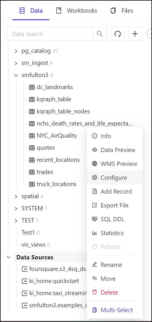
- The Edit Table panel will appear.
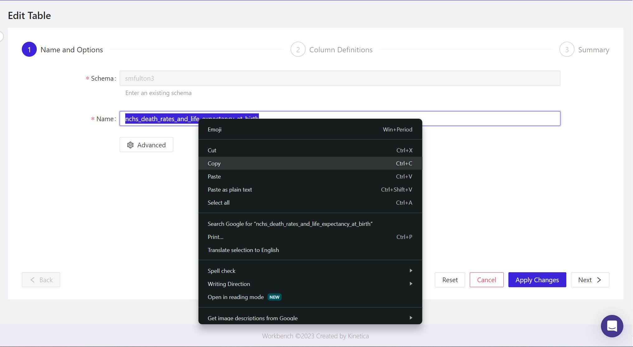
- In the Name field, highlight the complete table name, then in your browser, right-click and from the popup, select Copy.
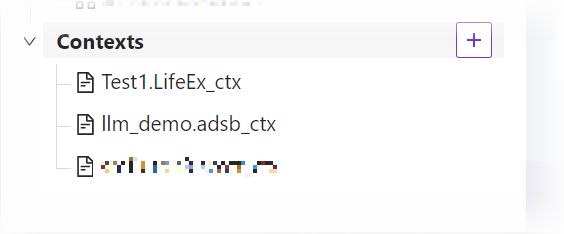
- In the Data tab, at the bottom of the list of database objects, click the + button beside Contexts. The Create Context panel will appear.
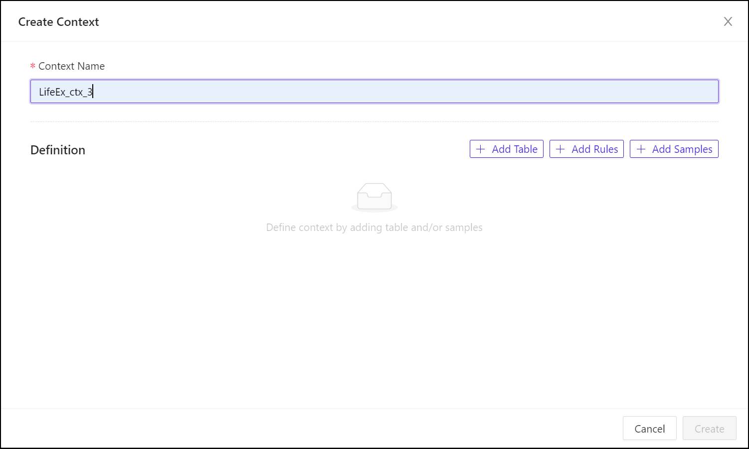
- In the Context Name field, enter a name for the context object in the database, using only letters, digits, and the underscore (_) character. This will be the name Kinetica will use to refer to the context.
- A context may refer to more than one table in a schema and you should add each table that the LLM should consider in responses. To begin associating a context with a table, click + Add Table.
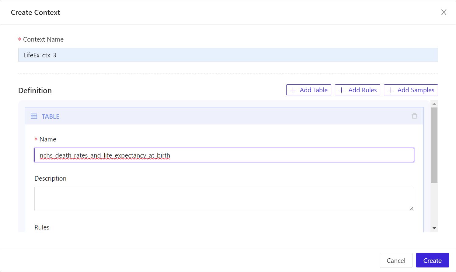
- In the Name field, enter or paste the name of the table you copied earlier.
- Under Description, type a sentence or phrases that describes the data in this table, making sure you use language and terminology that would likely be included in natural-language questions that refer to this data.
- Rules are optional within contexts, but very helpful. To add a rule that applies to a table, under Rules, click + Add Rule (you may need to scroll down) then enter the rule into the field that appears above the button.
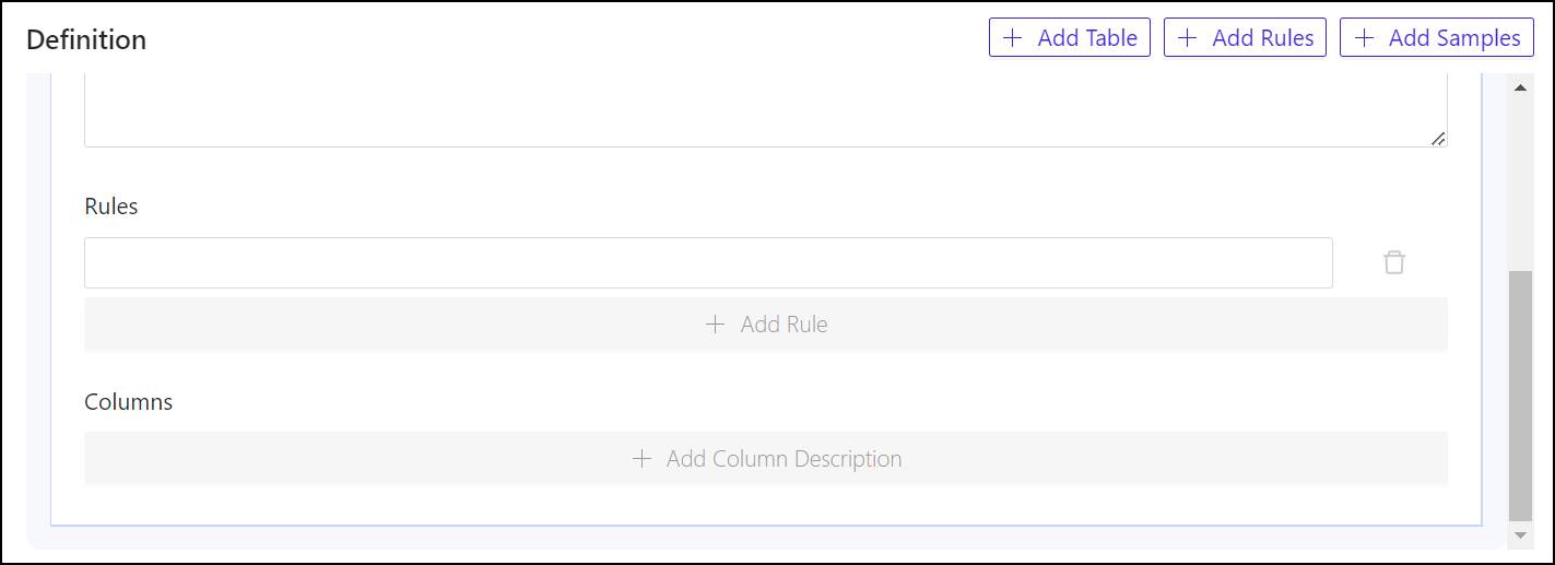
- Column descriptions are also optional, although they’re frequently necessary to give the language model enough synonyms and associated terms to deduce references to these columns from regular phrases. To add a column description for a column, click + Add Column Description. In the Name field, enter the exact field name for the column you wish to describe. Then under Description, enter a phrase that includes terms and words that are synonymous with that field name, and that would describe it adequately for a human user. Repeat this process for as many columns as may require descriptions.
- To add a rule that applies to the context or the schema as a whole, from the top of the Create Context panel, click + Add Rules. This opens up a Rules box toward the bottom of the set (you may need to scroll down to see it). To add the first rule, click + Add Rule, then enter the general rule into the field that appears above the button. Repeat for as many rules as your schema may require.
- To add one or more sample pairs, from the top of the Create Context panel, click + Add Samples. A box marked Samples will appear below the Rules box you opened earlier. To add the first sample in the set, click + Add Sample. Then under Question, enter a natural-language question you believe a regular user would pose. Under Answer, enter the SQL code that you know would yield the results that would satisfy this question. (You may wish to open a separate Kinetica workbook, to try SQL statements yourself until you get the results you’re looking for, then use the best statement as your answer for the sample.) Repeat for as many samples as you believe would best benefit your context.
- When you have populated the context components with enough clues, instructions, and samples, click Create. Kinetica will process your instructions as context creation statements, and will soon inform you of its results.
STEP 3: Ask SQL-GPT Questions
Now let’s test Kinetica’s SQL generation processes at work. Here, you’ll be creating a workbook in Kinetica Workbench that accepts your natural-language questions, and produces SQL statements you should be able to use in the Kinetica database. Here’s how to begin a new workbook:
- From the left pane of Kinetica Workbench, click Workbooks.
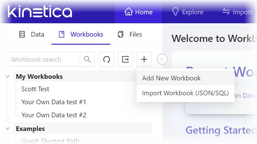
- From the Workbooks tab, point to the + button and from the dropdown, select Add New Workbook. The Create Workbook panel will appear.
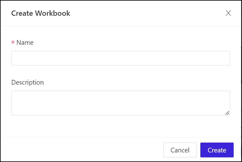
- Under Name, enter a unique name for the workbook. This is not a database object, so it can have special characters, distinguished upper and lower case, and spaces.
- Under Description, enter something that describes the purposes of the workbook for your purposes. This is not a description for a language model or for generative AI training; it’s just for you.
- Click Create to generate the workbook. It will soon appear in the Workbench window, and the first worksheet, named Sheet 1, will already have been generated.
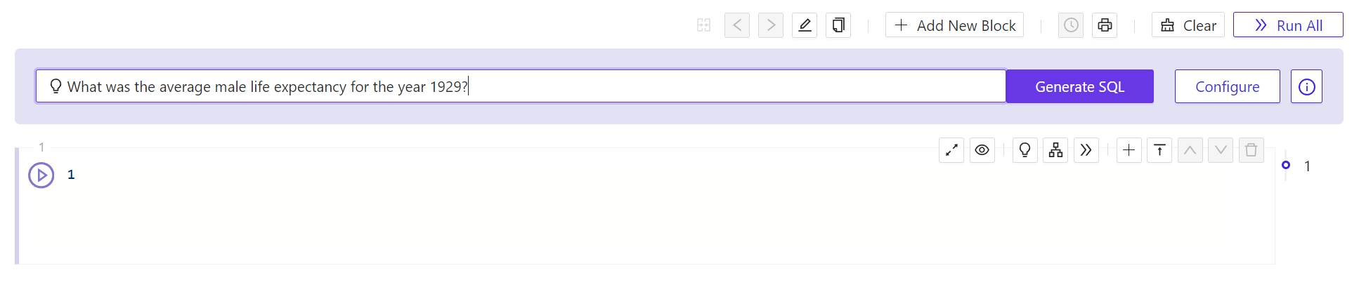
- In the field at the top of the panel marked with a light bulb, enter a natural-language question to which you’d like the database to be able to respond. You don’t need to include any extra syntax, such as quotation marks or SQL reserved words. Just type a question as though you were entering it into an AI chat window, then click Generate SQL. The Workbench will respond with a warning and the Context Configuration panel.
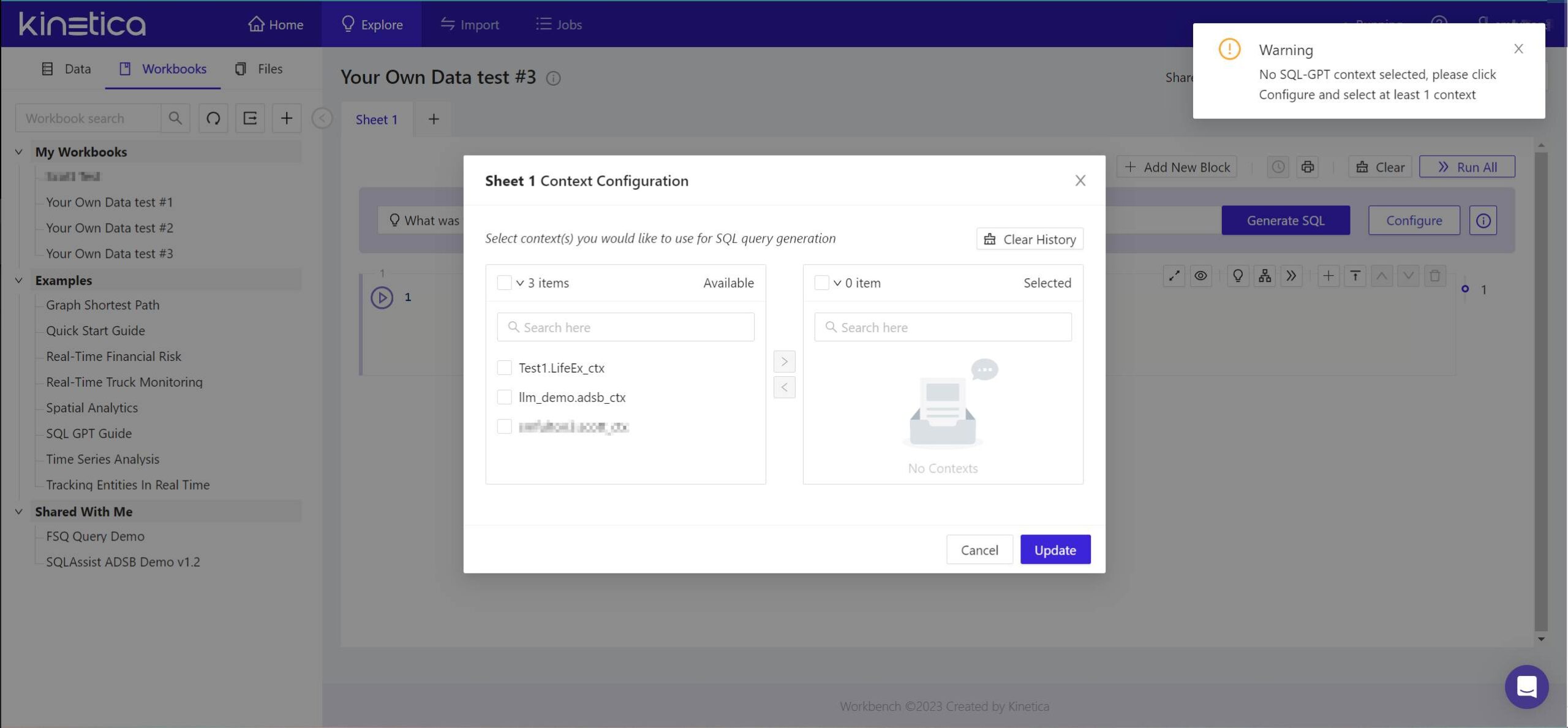
- The warning you will see indicates that Kinetica has not yet attached a context to the question you’ve posed. From the panel that appears, in the left-side list, check the box beside the name of the context you created earlier. Then click the > button so that it appears in the right-side list. Then click Update.
- After the panel disappears, click Generate SQL again. In a few moments, Kinetica will respond with a SQL statement. Its first line will be a comment containing the text of the question you posed.
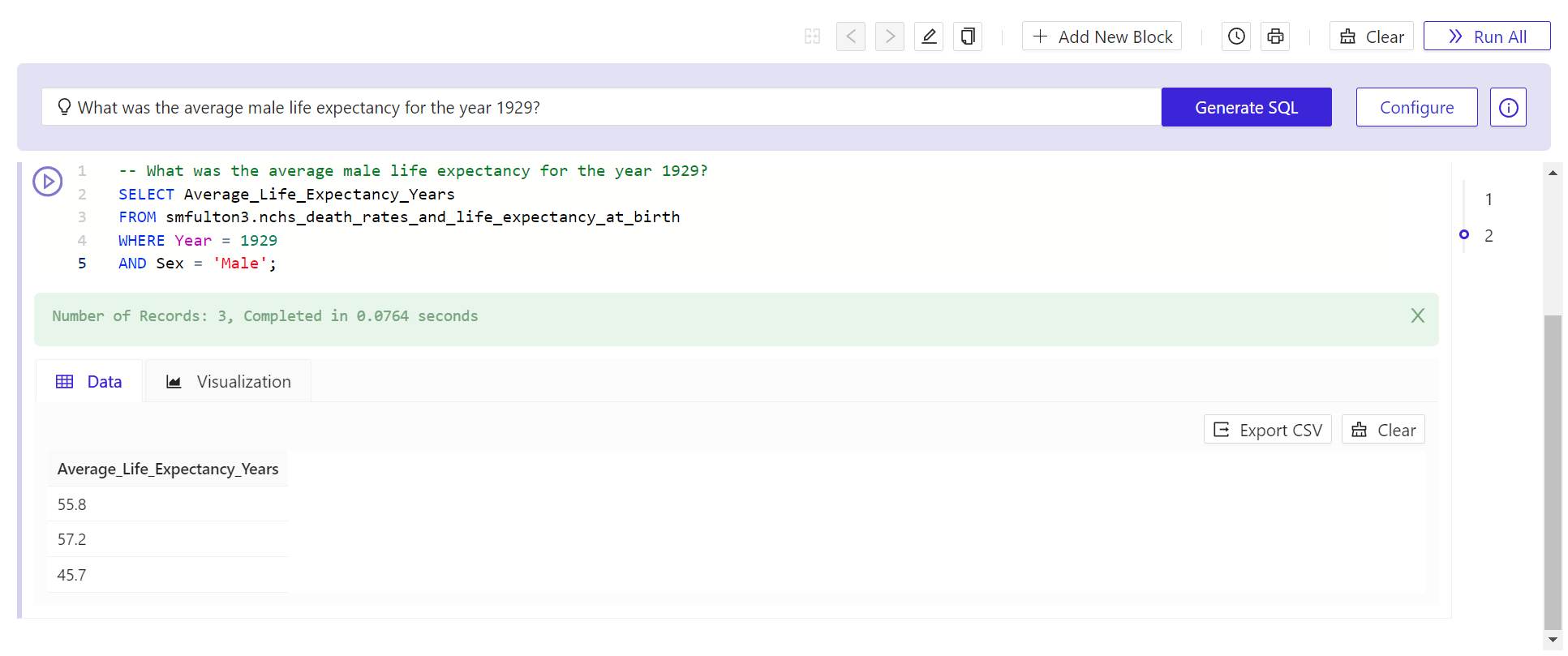
- To test this query on the data you’ve generated is to click the round > (Play) button to the upper left of the new query. In a very brief moment, Kinetica should respond with a view of data queried from the table or tables you imported.
It’s fair to say at this point, especially at the first go, that Kinetica may respond with something else: perhaps an error, or maybe data that does not actually resolve the criteria. Artificially intelligent inferencing is not a perfect process. However, you can improve the efficiency of the results by adding information to your context and trying again. It may take a few runs to get the correct results. Keep in mind, as you’re doing this, that the minutes you’re spending improving the language model’s ability to ascertain what your language is trying to say, equate to days and even weeks of work in a conventional ETL project, where engineers work to make databases more responsive to dashboards and ad-hoc queries in real time.
The post How to deploy natural language to SQL on your own data – in just one hour with Kinetica SQL-GPT appeared first on Kinetica - The Real-Time Database.
]]>The post The mission to make data conversational appeared first on Kinetica - The Real-Time Database.
]]>Kinetica provides a single platform that can perform complex and fast analysis on large amounts of data with a wide variety of analysis tools. This, I believe, makes Kinetica well-positioned for data analytics. However, many analysis tools are only available to users who possess the requisite programming skills. Among these, SQL is one of the most powerful and yet it can be a bottleneck for executives and analysts who find themselves relying on their technical teams to write the queries and process the reports.
Given these challenges Nima Neghaban and I saw an opportunity for AI models to generate SQL based on natural language, to give people immediate insights.
Where to begin
Initially we had no large language model (LLM) we could use, and I needed a proof of concept. I started with the OpenAI Playground, which provides tools for developing applications based on OpenAI and uses the ChatGPT LLM. With this, I was able to create a prompt that would generate SQL based on one of our sample schemas. Next, I worked with a UI developer to extend the Kinetica Workbench application so it could populate the prompt with the necessary schema details and send requests to the OpenAI API.
Our first release relied on the OpenAI LLM to generate SQL. We soon realized it had limitations, and many of our largest customers could not take full advantage of it. For example, many organizations can’t send proprietary data to a third party like OpenAI. In addition, the OpenAI models would often unexpectedly change results without explanation. There were many types of optimizations that would be helpful for efficient code generation, but they were not supported by OpenAI because it had not been optimized for generation of creative text. .
We understood that, to make this capability feasible for all our customers, we would need to develop a model that we had full control over.
Thinking like the startup we still are, we acquired some GPU’s off eBay that I put to use for fine-tuning a model. I wanted a model that was specifically trained for SQL generation, so I used some techniques not available with OpenAI. There are custom tokens for identifying SQL context, user, and assistant sections of the prompt. The training data uses masks to allow the optimizer focus on solutions for the SQL generation while using the other sections as preconditions.ChatGPT uses a relatively simple algorithm for inferencing that is more useful for creative writing than code generation. For the Kinetica model, I chose a deterministic algorithm called beam search that evaluates multiple solutions before choosing the best one. I also created a custom UI for developing and testing prompts under different conditions of inferencing parameters. This helped root out problems, and gave me an understanding of what worked best.

Contexts in context
In my previous installment, I brought up the subject of the context — a unique concept that the Kinetica namespace treats as a first-class object. I offered an analogy where I compared an LLM’s context to a human brain’s short term memory. During inferencing we use a strategy called in-context learning that provides a means to to give an LLM extra instructions without the need to run a compute intensive fine-tuning process..
In the Kinetica model, a context is currently limited to about 8,000 tokens, with each token representing 3 or 4 characters. Future LLM architectures may be able to handle longer contexts, which would free them to learn more continuously. Right now, an LLM is usually suspended in a frozen state after training, and it has its contexts wiped after each inference session.
At Kinetica, we developed a SQL syntax residing within the database to represent the data that we load into the context during the inferencing process. Then I developed an API endpoint to service the inferencing request coming from the database. The end result is a generative AI capability integrated into our core database, with first-class objects manipulated like any other database object.
Touchy subjects
Some users expect magic from the LLM when they ask the model to generate SQL for questions for which it does not have the data. In many cases, the model is working on proprietary customer data that was nowhere in its training.
I like to compare this task to asking a programmer/analyst to write SQL based only on the information in the context. How likely would a human successfully write a SQL instruction, without having seen the schema or data? You may have had an experience with a new coworker where you assign them a task, and they tell you they don’t understand something, or there’s a piece of information missing somewhere. Sometimes their sentiment is justified.
An LLM is trained to always respond with the result with the highest probability of being correct. Because of this, it can’t give you direct feedback about how, why, or where it’s confused — say, for instance, “I don’t know how to join this table, because I am not sure which term is the foreign key.” Instead, we have to infer the nature of the problem an LLM is having, solely from the erroneous responses we receive.
When used correctly, the LLM can seem surprisingly smart about what it can figure out for itself. Still, you still need to be thoughtful about what it needs to know. I can recall a number of times when I got frustrated trying to make it do something, and then I realized I gave it an incorrect example.
For this reason, among others, training data needs to have high quality and be unambiguous. Some studies have shown that, if you train a model with high-quality curated data, you need only a small fraction of what would otherwise be required to achieve a desired level of performance. If a training sample gives an incorrect answer, the model can get confused when it tries to correlate that answer with other correct answers — which leads to performance degradation. And if the question/answer pair includes an ambiguous question, the model may confuse the response as the answer for a different, but similar, question.
There is also this notion that LLM multitasking can degrade performance. For example, if you ask ChatGPT to answer a question while doing something trivial like capitalizing every noun, it might give lower-quality answers. When a model generates SQL, we want to keep its attention on generating a query that will produce a correct result. When it divides its attention on how best to format the code, or it sees samples in its context showing a number of ways to do the same thing, then it gets distracted. So it’s good to consistently format samples, and avoid using different varieties of syntax when just one will suffice.
All this raises some very interesting questions about how we could enhance LLMs in the future. Right now, LLMs don’t really learn by doing, but they could if we integrated a process capable of generating new training data, based on feedback from human users. By indexing successful samples with embeddings, we could give the LLM its own long-term memory, so it could improve over time.
The post The mission to make data conversational appeared first on Kinetica - The Real-Time Database.
]]>The post Towards long-term memory recall with Kinetica, an LLM, and contexts appeared first on Kinetica - The Real-Time Database.
]]>It seemed like a sensible enough stance to take, given that I spent the bulk of a typical work week translating ambiguous requirements from customers into unambiguous instructions a computer could execute. Algorithmic neural networks had been around since the 1950s, yet most AI algorithms had been designed to follow a fixed set of steps with no concept of training. Algorithms are sets of recursive steps that programs should follow to attain a discrete result.
While machine learning does involve algorithms at a deep level, what the computer appears to learn from ML typically does not follow any comprehensible set of steps. ML is a very different world. Once an ML system is trained, unlike an ordinary algorithm, it isn’t always clear what those steps actually are.
Re-envisioning
The whole approach to algorithms in AI changed in 2012, when a University of Toronto computer science team led by Prof. Geoffrey Hinton used GPUs to train deep neural networks, as part of a computer vision competition. Their model for rectified linear activation beat the competition by a long shot. By the next year, a majority of competitors had already abandoned their procedural algorithms and used deep neural networks.
I think the most interesting result of the discovery is that it was completely unexpected. For years prior, well-funded corporations had the resources available to them to train a model like that. Sure, there were neural networks, but they were only exhibiting success on a very small scale.
You could make a similar case about the development of the Transformer architecture in 2017, and GPT-3 in 2020. Up to that point, the most powerful language models used LSTM networks, though they could not scale upward after a few million or so parameters. GPT-2, an early transformer model, was impressive enough, yet it did not seem revolutionary. Some people at OpenAI had a “crazy” idea that if they spent $5 million upgrading GPT-2 (1.5 B parameters) to GPT-3 (175 B parameters), it would be worth the investment. They couldn’t have known in advance what the payoff would be. Yet their results were astonishing: The GPT-3 model exhibited emergent traits, capable of performing unanticipated and unforeseen tasks that weren’t even being considered for GPT-2.
The way all these events unfolded caused me to re-evaluate what I thought was possible. I realized there were many things we don’t understand about large ML models: for example, how when they’re given a large enough number of parameters, suddenly they exhibit emergent traits and behavioral characteristics. When a large language model exceeds about 7 billion parameters, for some reason, it behaves differently. We don’t have any workable theories about why this happens. And we don’t yet have a good way to predict how or when these capabilities will suddenly change.
So many products and platforms have aimed to reduce or even eliminate the need for coding — Business Objects, PowerBI, Tableau, and all those “fourth-generation languages.” Yet once you’ve successfully “integrated” these tools into your workflow, they become bottlenecks. They require decision makers to build the skills necessary to use them effectively – or else wait for analysts or data scientists to come in, analyze how they’re being used, and write their own reports. Still, I saw the potential for generative AI to empower anyone in an organization to query a database which would enable users to get otherwise inaccessible insights.
Associations and contexts
To better understand how AI handles semantics — the study of the meaning of words — we should turn our attention for a moment to the human brain. In the study of neurology, semantics has been shown to have a definite, if unexplained, connection to people’s short-term memory. The effectiveness of semantics in aiding recall from short-term memory, appears to be limited.
Consider a situation where you get an email from someone you haven’t seen in ten years or so. You can be looking at their name, and gleaning a few details about them from the message. But you could be stuck trying to recall their identity from your long-term memory, until you gather enough information about them from the message to trigger an association. Short-term memory works sequentially, but long-term memory works through connections. Sometimes it takes time for your short-term memory sequences to build enough connections to serve as a kind of context, that would trigger your long-term memory associations.
An LLM has its own context that’s analogous to a person’s short-term memory. The size of this context is limited, since the computation requirements of Transformer models scales quadratically with the context’s length. It’s important for us to use contexts effectively, because they enable us to train the model for any given, specific inferencing query in a few seconds’ time, without needing to optimize and update the 16 billion parameters that comprise the model.
Today, Kinetica is working on a vector capability that will create an index of embeddings, that collectively represent semantic bits of information that can be easily modified. These embeddings may represent many different types of data, including natural language, stock market data, or database syntax. Using an LLM to recall information associatively, we can augment the context with information retrieved from a semantic search, then place the results from that search inside context objects. Then with an inferencing request, we would query the index using a semantic similarity search, and then use the results to populate the short-term memory represented by the context. The results we expect to see will be the type of associative recall of information, events, and even complex concepts that could never be attained from ordinary semantic search processes, like the typical Google search.
The evolutionary issue
Speaking for myself, I still maintain a healthy level of skepticism about the capabilities of modern AI systems. You won’t see me jumping onto Elon Musk’s anti-AI bandwagon, or signing a petition to pause or halt AI research. I believe humanity to be a far greater threat to itself than AI, and elevating AI to the level of an existential threat is a distraction from far more important issues that we face.
That being said, the swift emergence of generative AI makes me wonder if we could create an LLM with the capacity for a large, persistent, and evolving context. Such a data construct would have the ability to retain long-term memories, pose new questions of its own, and explore the world around it. Of course, such an AI would have an ability that no system has today: the ability to evolve its own capabilities independently of outside programming or influence. Normally, such a development would sound like it’s a long way off. But considering the history of unexpected advancements, I’ll say instead: Stay tuned.
The post Towards long-term memory recall with Kinetica, an LLM, and contexts appeared first on Kinetica - The Real-Time Database.
]]>The post Conversational Query with ChatGPT and Kinetica appeared first on Kinetica - The Real-Time Database.
]]>Warning: Undefined array key "file" in /home/yiplnet/kinetica.yipl.net/wp-includes/media.php on line 1763
Deprecated: preg_match(): Passing null to parameter #2 ($subject) of type string is deprecated in /home/yiplnet/kinetica.yipl.net/wp-includes/media.php on line 1763
Step 1: Launch Kinetica
Kinetica offers a “free forever” managed version with 10 GB of storage that is hosted in the cloud. It takes about two minutes to launch and only requires an email address to sign up. You can access it through this link and follow the instructions to create an account and launch Kinetica.
Step 2: Open the Quick Start Guide Workbook and Load Taxi Trip Data
Workbench is Kinetica’s primary user interface for analysts, data scientists and data engineers. It helps you manage data, files and SQL workbooks and perform administrative tasks. Workbooks provides an environment for querying and visualizing your data. I will be using the Quick Start Guide workbook to get started. For those of you who have used Kinetica in the past and are logging back in, make sure to refresh the examples before you open the Quick Start Guide workbook so you get the latest version that is configured for ChatGPT.
The Quick Start Guide workbook uses the New York City taxi data to show Kinetica’s analytical capabilities. Run all the SQL query blocks in the “1. Load the data” worksheet. The two tables we are interested in for this tutorial are:
- The taxi trip data (“taxi_data_historical”) that contains information about taxi trips.
- The spatial boundaries of different neighborhoods in New York City (“nyct2020”).

Step 3: Try out a Sample Prompt in the ChatGPT Sheet
All workbooks in Kinetica now have a chat prompt. You can use this prompt to send analytical questions in plain English to ChatGPT. This will return a SQL query that references data in Kinetica, which is added as an executable code block to your worksheet.

In the instance above, we have asked GPT to identify the total taxi drop-offs by each vendor to JFK airport in New York City. It returns a query that
- Identifies the spatial boundary for JFK airport using the nyct2020 table.
- Filters all the records where the drop-off longitude and latitude from the taxi trip data was contained within the spatial boundary for JFK airport identified in Step 1.
- Summarizes the total trip by the vendor ID to calculate the drop-offs at JFK airport.
SELECT "vendor_id", COUNT(*) AS num_trips
FROM "taxi_data_historical"
WHERE ST_CONTAINS(
    (SELECT "geom" FROM "nyct2020" WHERE "NTAName" = 'John F. Kennedy International Airport'),
    ST_MAKEPOINT("dropoff_longitude", "dropoff_latitude")
)
GROUP BY "vendor_id"
This is not a simple query to execute, particularly on billion-row datasets. But because Kinetica has a highly performant vectorized query engine, it can execute these ad hoc queries on large amounts of data without any additional setup or pre-processing of the data. Head over to the “ChatGPT” worksheet to try out a few of the sample prompts listed there.
Step 4: Configure Chat Context
There are a few things to keep in mind when using the chat feature. The first is that we need to provide ChatGPT with enough context about the data so that it can generate queries that are specific to the tables inside Kinetica. We can do this by configuring the chat context.
The first part of the configuration describes the tables in plain English. The Quick Start Guide already includes this configuration, but if you want to try it yourself with your own data or a different table, you will need to configure the context yourself. Here I am describing the taxi trip and neighborhoods table that we queried just now. Behind the scenes, Kinetica also provides GPT with the data definition for each table. The data definition language (DDL) taken together with the description here provides enough context to GPT for it to generate meaningful queries that are specific to the data. Note that Kinetica does not send any data to ChatGPT, only metadata about the tables (DDL), such as column names and types.

In addition to describing the tables, we can also specify comma-separated rules. Rules are a way to further refine query outputs from ChatGPT. These can include things that are specific to Kinetica or your own preferences for how the queries should be constructed.
In my experience, the best way to configure rules is by trial and error. Try out a few different prompts and examine the queries that are returned. If you notice that something could be improved, then add that as a rule.
For instance, if we delete the rule that asks GPT to use full names of neighborhoods and rerun the same prompt we provided it earlier, we will get a slightly different query with a shortened version of the name “JFK airport” instead of “John F. Kennedy airport.” This query will run, but it will not yield the expected result because a neighborhood with this shortened name does not exist in the nyct2020 table.

Step 5: Create Your Own Workbooks, Load Your Own Data and Write Your Own Prompts
Now you can start writing your own prompts to query your data. Create a workbook using the plus icon on the workbook tab. Use the import tab at the top of the page (next to Explore) to connect to hundreds of different data sources and load data from them into Kinetica.
Be sure to configure your chat so that ChatGPT knows about the DDL for the tables you plan to query.
Writing Prompts Is More an Art Than a Science
As with human conversations, there is some variability in the responses that we get from ChatGPT. The same prompts with the same context could yield different results. Similarly, prompts with slightly altered wording can change the SQL query that ChatGPT returns.
So make sure to check the queries generated to ensure that they make sense and that the results are what you expected.
Try It out for Free
This workbook is now available as a featured example that you can access for free using Kinetica Cloud. It takes just a few minutes to create an account and launch Kinetica. Go ahead and give it a whirl.
The post Conversational Query with ChatGPT and Kinetica appeared first on Kinetica - The Real-Time Database.
]]>The post Using Window Functions in SQL appeared first on Kinetica - The Real-Time Database.
]]>A window function performs a calculation across a set of rows that are related to the current row, based on a specified window of observations. They are used to calculate running totals, ranks, percentiles and other aggregate calculations that can help identify patterns or trends within groups. Let’s look at how to use window functions in SQL.
The code below shows a moving average calculation that uses a window function. It applies the average function over a window with five observations that is partitioned by a stocks symbol and ordered by time.
AVG(price_close) OVER (
    PARTITION BY symbol
    ORDER BY time
    ROWS 5 PRECEDING
) AS avg_price
Let’s break this down to understand the purpose of each of these clauses.
Apply Function OVER a Window
At the most abstract level, we can think of a window function as being applied on a “window” of rows that are related to the current row. The specified window slides with the “current row” so that the set of values that a window function is applied to updates with each row (see animation below). The window function generates one result value per row thereby allowing us to preserve the original granularity of the data.
The window function above calculates the rolling average price for the past five observations using a window for the AAPL (Apple) stock price.

This is a simple illustration of a window function. It works because the rows in the table are ordered by the time column and because the only stock symbol is AAPL so the previous five rows correspond to the last five observations of AAPL.
But what if the rows in the table were not ordered by the timestamp? Or if there were other stock symbols in the table. These cases are handled using the ORDER BY and PARTITION BY clauses in the window function. Let’s explore these next.
ORDER BY
The animation below illustrates the ORDER BY clause. The table is initially not ordered by the timestamp column. As a result, the average is not being computed on the previous five observations. We can fix this by simply ordering the data on the time column. Note that the window function does not update the actual ordering of the table itself, it simply reorders the rows for the sake of performing the calculation without mutating the table itself. This is important since it doesn’t inadvertently affect other queries that might require the table to be ordered on a column other than time.

Now, let’s introduce another layer of complexity. Imagine that the table includes two additional stock symbols — GOOG (Google) and AMZN (Amazon).
PARTITION BY
We can address this by partitioning the data on the stock symbol column.

By partitioning the data by each stock, we apply the window on observations within each partition rather than across them. Note that just like the ordering clause, partitioning the table does not replace the structure of the input table.
The final piece in a window function is the sizing of the window itself — the “frame.”
Framing a Window
So far, we have positioned the window above the current row with an arbitrary number of rows as its size. But what if we wanted to position the window elsewhere (above the current row, including the current row, from start, etc.)? The frame clause inside a window specification offers a great deal more flexibility and control over the sizing of a window.
There are two types of frame clauses, rows and range. A range clause considers the values of the records in the ordering column. While a row clause considers the ordering of the records. This can be a bit hard to understand when written down but the distinction between the two crystallizes when we encounter duplicate (or “peer”) values in the ordering column.
The tables in the illustration below have duplicate values in the ordering column time. Let’s ignore the partitioning for now. A row clause that specifies a frame with one row preceding and following the row will result in a frame with three observations in it — the row preceding the current row, the current row and the row following the current row. The range clause on the other hand yields a window that has nine rows in it — all the records with value of time (the ordering column) that fall within a range one less than or one more than the time of the current row. This includes all records with a time in the range 9:42 to 9:44

There are a few options when setting the start and end points for a frame. These are listed below along with their description.
Frame start keywords |
UNBOUNDED PRECEDING | The first row of the partition |
| <number> PRECEDING | Either n rows before the current row (for rows-based frames) or n values less than the current row’s value (for range-based frames) | |
| CURRENT ROW | Either the current row (for rows-based frames) or the current row and its peer rows (for range-based frames) | |
| <number> FOLLOWING | Either n rows after the current row (for rows-based frames) or n values greater than the current row’s value (for range-based frames) | |
Frame end keywords |
UNBOUNDED FOLLOWING | The last row of the partition |
| <number> FOLLOWING | Either n rows after the current row (for rows-based frames) or n values greater than the current row’s value (for range-based frames) | |
| CURRENT ROW | Either the current row (for rows-based frames) or the current row and its peer rows (for range-based frames) | |
| <number> PRECEDING | Either n rows before the current row (for rows-based frames) or n values less than the current row’s value (for range-based frames) |
Now, let’s check out a few examples for common window function queries.
A Moving Average with Row-Based Frames
The query below is an illustration of a simple moving average. The partition by clause separates the rows based on the stock symbol, the ordering clause arranges the rows within each stock partition in descending order of time, and the row clause specifies a window frame with five observations before the current row.
SELECT
    time,
    symbol,
    AVG(price_close) OVER
        (
            PARTITION BY symbol
            ORDER BY time
            ROWS 5 PRECEDING
        ) AS mov_avg_price
FROM trades
A Moving Average with Range-Based Frames
The query below is similar to the one above but with one important difference. We are using a range-based frame instead of a row. The range clause specifies a frame with all observations that have a time value within five minutes (300,000 milliseconds) of the current row. This includes observations before and after the current row.
SELECT
    time,
    symbol,
    AVG(price_close) OVER
        (
            PARTITION BY symbol
            ORDER BY time
            RANGE BETWEEN 300000 PRECEDING AND 300000 FOLLOWING
        ) AS mov_avg_price
FROM trades
Ranking
So far we have seen aggregate functions that summarize the observations in a particular window frame. Ranking functions comprise another type of window functions. They are used to compare data points within a given series or between different series and determine their relative importance. In the query below, I am using a ranking function to rank the closing prices of different stocks. Notice how the ordering column is now the closing price and not time. This is because the rank is determined based on the ordering column.
SELECT symbol, time price_close,
    RANK() OVER (
       PARTITION BY symbol
       ORDER BY price_close DESC
    ) AS high_price_rank
FROM trades
ORDER BY high_price_rank
Try This on Your Own
Kinetica offers 18 different window functions (aggregate + ranking). And the time series workbook contains several window functions and it is a good starting point.
You can import this workbook into Kinetica Cloud or Kinetica’s Developer Edition to try these out on your own. I have pre-configured all the data streams so you don’t have to do any additional setup to run this workbook.
Both Kinetica Cloud and Developer Edition are free to use. The cloud version takes only a few minutes to set up and it is a great option for quickly touring the capabilities of Kinetica. The Developer Edition is also easy to set up and takes about 10 to 15 minutes and an installation of Docker. The Developer Edition is a free forever personal copy that runs on your computer and can handle real-time computations on high-volume data feeds.
The post Using Window Functions in SQL appeared first on Kinetica - The Real-Time Database.
]]>The post How to Build Real-Time Location Intelligence Apps appeared first on Kinetica - The Real-Time Database.
]]>Over the past few years, building real-time location intelligence solutions has become easier thanks to the introduction of new specialized technologies that are designed to handle the processing, analysis and visualization of location-based data.
In this article, you will learn how to set up a location intelligence pipeline that is built on top of real-time data feeds from Apache Kafka. The workbook contains an end-to-end pipeline that connects to streaming data sources via Kafka, performs spatial computations to detect different events and patterns, and then streams these to an external application. All of this is done using simple SQL code without any need for complicated data engineering. You can follow along using the Kinetica workbook in this link.
Setup
There are a few things to consider when picking a database for real-time spatial analysis.
- Native connectors to streaming data sources like Kafka
- Functional coverage: The ST_Geometry library from PostGIS is the gold standard for geospatial functions. Most spatial databases emulate this library.
- Spatial joins: The ability to combine multiple tables based on a spatial relationship. This is important for any type of sophisticated analysis of spatial data.
- Performance: Real-time applications require spatial functions to be executed on large amounts of data at high speeds.
- Reactivity: The system needs to automatically detect and respond to new data without any elaborate engineering on our part.
- Integrated capabilities: Location intelligence workloads often have niche analytical requirements such as routing and optimization using graph networks and the ability to visualize large amounts of data.
- Stream data out: The final piece of the pipeline is the ability to stream data out of an analytical database into external systems.
This demo uses Kinetica’s free developer edition to run the queries in this article. See the last section of this article for more information on how to try the queries here on your own.
Data
We will use the following data for this demo.
- A stream of GPS coordinates that record the movement of seven trucks in Washington, D.C. The data is being streamed in via a Kafka topic.
- A set of polygons that outline different landmarks in D.C.
- A stream of taxi trips that are occurring in New York City (a few hundred per second)
All the data feeds are preconfigured so you don’t have to do any setup to replicate the queries here on your own. The maps below are a visual representation of the data.


Let’s dive into a few common analytical tasks that underpin location intelligence.
Spatial Filtering
A spatial filter is used to identify a subset of records from a table that meet some criteria based on a specific spatial query.
Let’s start with a really simple query to kick things off. The query below, identifies all the “fences” — the outlines around landmarks that have an area greater than 0.5 km2 (500,000 m2).
CREATE OR REPLACE TABLE fence_filter AS
SELECT wkt
FROM dc_fences
WHERE ST_AREA(wkt, 1) > 500000
This is a pretty easy query to implement in any database that supports spatial operations since it is filtering from a small table. Now let’s explore a few use cases that are harder to implement in real time.
Spatial Join of Streaming Locations with the Fences Table
Spatial joins combine two different tables using a spatial relationship. They are used to answer questions such as “which areas overlap,” “where do the boundaries occur” and “what is the area covered by a certain feature.” Spatial joins are typically computationally expensive to perform, especially on larger data.
The query below performs an inner join between the recent_locations table and the dc_fences table that outlines landmarks in D.C. based on the following criteria: Find all records where a truck came within 200 meters of a landmark in D.C.
CREATE OR REPLACE MATERIALIZED VIEW vehicle_fence_join
REFRESH ON CHANGE AS
SELECT
    TRACKID,
    x,
    y,
    DECIMAL(STXY_DISTANCE(x, y, wkt, 1)) AS distance,
    fence_label,
    wkt
FROM recent_locations
INNER JOIN dc_fences
    ON
    STXY_DWITHIN(x, y, wkt, 200, 1) = 1;
Everything looks similar to PostGIS but …
This query looks remarkably similar to any query that you might see in PostGIS or any other spatial database that uses ST_Geometry. The key difference, however, is the use of the materialized view that is set to refresh on change. This means that the query will be updated in real time as new records with truck location hit the Kafka topic.

With this change, the database will constantly monitor and maintain the join view (vehicle_fence_join) to reflect the most up-to-date version of truck locations. Or in other words, if there is a new truck location that is close to a landmark, it will be automatically reflected in the join view.
Take It up a Notch with a Time Filter
In the previous query we identified all the records that matched spatial criteria. Now, let’s add time-based criteria.
The query below identifies all instances from the last 5 minutes where a truck location was inside one of the “fences” around a landmark in Washington, D.C.
CREATE OR REPLACE MATERIALIZED VIEW fence_events
REFRESH ON CHANGE AS
SELECT
    TRACKID,
    wkt,
    x,
    y,
    TIMESTAMP,
    CONCAT(TRACKID, CONCAT(' is at ', fence_label)) AS event_text
FROM recent_locations, dc_fences
WHERE
    STXY_CONTAINS(wkt, x, y) = 1 AND
    TIMEBOUNDARYDIFF('MINUTE', TIMESTAMP, NOW()) < 5
The query above performs a very common location intelligence task: geofencing. Geofencing is a location-based service in which a software application uses GPS, RFID, Wi-Fi or cellular data to trigger a preprogrammed action when an object enters or exits a virtual boundary set up around a geographical location. Geofencing can be used for various purposes, such as sending notifications to customers when they enter or leave an area, providing targeted advertising based on location, and tracking employee time and attendance.
Now, there is one particular scenario where the query we used above will fail. Consider a fence that is really small; an object might enter this fence and then subsequently exit before it emits a location signal. Or in other words, if we don’t have data on a geofence event, we won’t be able to detect it.
But there is a workaround for this. We can interpolate the “track” between two subsequent points to then infer if the track intersects with the fence. Let’s look at that next.
Add Interpolation with Tracks for More Accurate Detection
The animation below shows the scenario we just described. Without interpolation it might seem that a particular object did not enter a fence. But with interpolation, we can correctly infer that the track did indeed intersect with a fence.

Kinetica offers a native track object that does all the interpolation behind the scenes. A track requires the following information: a timestamp (so that we know the order of the points), the X and Y (longitude/latitude) coordinates of the object and an ID variable that identifies each track.
We can use this with the ST_TRACKINTERSECTS function to infer geofencing events as shown below.
CREATE OR REPLACE MATERIALIZED VIEW fence_trucks
REFRESH EVERY 5 SECONDS AS
SELECT *
FROM TABLE
(
    ST_TRACKINTERSECTS
    (
        TRACK_TABLE => INPUT_TABLE(recent_locations),
        TRACK_ID_COLUMN => 'TRACKID',
        TRACK_X_COLUMN => 'x',
        TRACK_Y_COLUMN => 'y',
        TRACK_ORDER_COLUMN => 'TIMESTAMP',
        GEOFENCE_TABLE => INPUT_TABLE(dc_fences),
        GEOFENCE_ID_COLUMN => 'fence_id',
        GEOFENCE_WKT_COLUMN => 'wkt'
    )
);
There are several other track functions that come with Kinetica, but you can try those out on your own using the workbook.
Binning and Aggregation
The final spatial operation I want to cover is binning and aggregation. We will use the stream of taxi trips from New York City for this section. This data contains information about the pickup and drop-off locations, fare and distance of each taxi trip in New York City. We are interested in finding hotspots in the taxi locations in the city.
Spatial binning is a technique used in data analysis to group geographically referenced data into user-defined bins or areas. The technique is used to reduce the resolution of a dataset, making it easier to visualize and analyze large datasets. This can be done by dividing the area into equal-sized rectangular grids, circles, polygons or hexagons. The resulting bins are then used for statistical analysis, such as calculating the frequency of events or measuring average values.

Kinetica offers multiple ways to generate grids for binning data: ST_HEXGRID or using H3 geohashing functions. Let’s use the latter.
Uber developed H3 (Hexagonal Hierarchical Spatial index) for efficiently optimizing ride pricing and visualizing and exploring spatial data. Each grid in the systems has an associated index and a resolution.
We can use the STXY_H3 function to identify the corresponding grid index value for each taxi drop-off and pickup location for the taxi data stream — into which hexagon a particular point falls.
Note that the materialized view is set to refresh on change, so as new data hits the system (a few hundred trips every second), the view below is automatically maintained by calculating the H3 index values for all the new records.
CREATE OR REPLACE MATERIALIZED VIEW nytaxi_h3_index
REFRESH ON CHANGE AS
SELECT
    pickup_latitude,
    pickup_longitude,
    STXY_H3(pickup_longitude, pickup_latitude, 9) AS h3_index_pickup,
    STXY_H3(dropoff_longitude, dropoff_latitude, 9) AS h3_index_dropff
FROM taxi_data_streaming;
Once we have the index values, we can use those to generate the corresponding bins using the ST_GEOMFROMH3 function. The data is then grouped by the index to calculate the total number of pickups in each bin. This is another materialized view that is listening for changes to the materialized view we set up in the query above. Again the aggregations are automatically updated and as new records arrive, the view will always reflect the most up-to-date aggregation without any additional work on our part.
CREATE OR REPLACE MATERIALIZED VIEW nytaxi_binned
REFRESH ON CHANGE AS
SELECT
    h3_index_pickup,
    ST_GEOMFROMH3(h3_index_pickup) AS h3_cell,
    COUNT(*) AS total_pickups
FROM nytaxi_h3_index
GROUP BY h3_index_pickup
The map below shows the results. We can see that the hotspots for pickup are mostly in Lower Manhattan.

Try This on Your Own
You can try all of this on your own for free using the Spatial Analytics workbook on Kinetica Cloud, or by downloading the workbook from our GitHub repo here and importing it into Kinetica’s Developer Edition. I have preconfigured all the data streams so you don’t have to do any additional set up to run this workbook.
Both Kinetica Cloud and Developer Edition are free to use. The cloud version takes only a few minutes to set up, and it is a great option for quickly touring the capabilities of Kinetica. However, it is a shared multitenant instance of Kinetica, so you might experience slightly slower performance.
The developer edition is also easy to set up and takes about 10 to 15 minutes and an installation of Docker. The developer edition is a free personal copy that runs on your computer and can handle real-time computations on high-volume data feeds.
The post How to Build Real-Time Location Intelligence Apps appeared first on Kinetica - The Real-Time Database.
]]>The post Unlock Opportunities with Continuously Updated Materialized Views appeared first on Kinetica - The Real-Time Database.
]]>As the underlying data changes, materialized views need to be refreshed to keep the data in the view up to date. But this can be a resource intensive process. Many databases struggle to to keep materialized views up to date with frequently changing data, or for views from complex queries with multiple joins, aggregations, and subqueries.
For instance, consider a data stream of thousands of retail transactions every second. A traditional materialized view that is built on top of this transaction stream might only be updated once every day, or perhaps even as infrequently as once a week – if the query is really complex. As a result, you end up with upstream dashboards and analytical tools that are not at pace with the real-time data feed.
Kinetica’s powerful vectorized engine removes this constraint, allowing you to build and maintain complex materialized views on data that is changing continuously. This allows for high volumes of concurrent users accessing a materialized view will always see the most up-to-date version of the results.
What is a materialized view?
Let’s first understand what a view is. SQL views are virtual tables that are a result of stored queries. They are like a normal table in the database and contain rows and columns of data, but the data is not physically stored in the database. Instead, when a view is called, it executes the query and returns the result set.
A materialized view is similar to a regular view in that it is based on one or more underlying tables, but the data in the materialized view is actually stored on disk like a regular table. This data can then be queried directly, without having to re-execute the underlying query.
Traditional databases cannot update materialized views continuously
Materialized views are typically used to improve the performance of queries that involve aggregating large amounts of data or joining multiple tables. Since the results of the query are already stored (and indexed) in a table, it can be accessed directly, rather than being computed on the fly each time the query is run.
But there is a flip side to this performance gain, which is the overhead of maintaining and refreshing a materialized view. This overhead depends on the complexity of the query that is used to create the view and the frequency at which it needs to be refreshed. It can be quite costly to maintain a materialized view if the underlying data is constantly being changed or updated.
The primary cost associated with maintaining materialized views is query execution time. If the query used to define the view is complex or requires cross-table joins, this can take considerable time to run every time the view needs to be refreshed. Additionally, if the underlying data changes often or there are frequent updates, it will take longer for the view to refresh as it must account for all of these changes each time it updates.
How does Kinetica maintain continuously updated materialized views?
Kinetica leverages its built-in vectorized and distributed query processing capabilities to blow through computational barriers and provide continuously updated materialized views.
Vectorization, to put it simply, is the ability to execute each instruction – like, say, adding two numbers – on multiple pieces of data at the same time. This is thousands of times faster than the traditional sequential mode of execution, where each piece of data is operated on in sequence, one after the other.

Sequential mode

Vectorized (Single Instruction Multiple Data)
These performance gains are substantiated by benchmarks that show that Kinetica is 8 X faster than Databricks 9.1 LTS (Photon), 50 X faster than Clickhouse and 240 X faster than PostGIS.
Kinetica has a vast library of in-database functions that are fully vectorized, and it has native connectors for streaming data sources like Kafka. This allows it to quickly process high frequency streaming data and run really complex vectorized queries that execute much faster than other databases. As a result, Kinetica can be used to set up always on analytical pipelines that keep materialized views continuously updated to always reflect the latest version of the data.
For instance, the query below, from one of our example workbooks, creates a materialized view that stores summary statistics about ship tracks in the Gulf of Mexico region. The underlying table for this query – ship_tracks – receives a few thousand records per second from a Kafka topic containing information on new ship locations. Notice the REFRESH ON CHANGE option, Kinetica is able to process all of this data and run complex geospatial queries to keep this view updated in real-time.
CREATE OR REPLACE MATERIALIZED VIEW track_summary
REFRESH ON CHANGE AS
   SELECT TRACKID,
          COUNT(*) AS n_obs,
          ROUND(ST_TRACKLENGTH(Y, X,TIMESTAMP, 1) / 1000) AS track_length_km,
          ROUND(ST_TRACKDURATION(HOUR,TIMESTAMP)) as duration,
          ROUND((ST_TRACKLENGTH(x,y,TIMESTAMP,1) / 1000)/ST_TRACKDURATION(HOUR,TIMESTAMP)) as avg_speed,
          MIN(X) AS min_longitude,
          MAX(X) AS max_longitude,
          MIN(Y) AS min_latitude,
          MAX(Y) AS max_latitude
    FROM ship_tracks
    GROUP BY TRACKID
    ORDER BY track_length_km DESC;
This is simply not possible with other technologies.
You can try this out for free by running the entity tracking example in Kinetica’s workbench. Alternatively, you can access the workbook and the code from our examples repo on GitHub.
Use-Cases for Continuously Updated Materialized Views
Kinetica’s ability to maintain complex materialized views on top of streaming data sources, opens up new possibilities.
- Real-time analytics and reporting: Materialized views enable users to quickly query and analyze large datasets in real time.
- Eventing systems: Kinetica’s wide range of in-database functions can be coupled with continuously updated materialized views to create always on eventing systems that detect events as they unfold and trigger downstream alerts.
- Real-time dashboards for data exploration: Dashboards and charts will always reflect the most current data and calculations. These are extremely useful for industries such as finance where analysts need to observe and respond to events in real-time.
- Machine learning models: One of the challenges with operationalizing machine learning models is the inability to serve the most up-to-date versions of complex derived variables to these models for inferencing. Continuously updated materialized views solve this problem.
- Replace traditional workloads: The computational constraints imposed by traditional databases are not an issue with Kinetica. So less performant materialized views from these databases can be boosted both in terms of performance and in terms of scale by switching to Kinetica.
Contact us
We’re a global team, and you can reach us on Slack with your questions and we will get back to you immediately.
The post Unlock Opportunities with Continuously Updated Materialized Views appeared first on Kinetica - The Real-Time Database.
]]>The post Optimizing Longer Routes for Electric Vehicles needing Charging Stations appeared first on Kinetica - The Real-Time Database.
]]>As of 2021 there are around 45,000 public outlets in the US. Pre-planning the most economical route can be a complicated algorithmic challenge, especially considering the various types of stations, availability and traffic conditions.
Kinetica’s graph route-solving capability can be used as the platform to calculate these optimal paths to minimize the total cumulative driving distance between the end points of a trip.
We needed a fast, practical and accurate graph-based optimization solver, with parameters specific to the optimal routing problem of an EV trip involving multiple charging stops so that different capacity limits and re-charging penalties can be rolled into the optimization algorithm
We surveyed various mapping and routing algorithms from Mapbox, Google, TomTom that are used by car manufacturers, such as BMW, Tesla, Hyundai, and Nissan. Many EV routing algorithms employ chronological shortest-path tree algorithms towards the same goal.
We devised a combinatorial optimization algorithm and a fixed storage graph topology construction for the graph road network of the continental USA. We re-purposed Kinetica’s existing Dijkstra solver to reduce the computational cost of many shortest path solves involved in the algorithm to meet SLA requirements. Our solution does not use bi-directional A-star Dijkstra between the prospective stations, and does not require finding a pivot location between charging locations.
An adaptive and light weight spatial search structure is also devised for finding a set of prospective stations at each charging location using uniform bins and double link associations. The entire algorithm is then implemented as yet another multi-threaded at-scale graph solver within the suite of Kinetica-Graph analytics, exposed as a restful API endpoint and operable within SQL.

This capability is demonstrated with example trips. See the results and get the details in the full paper: “Optimal routing algorithm for trips involving thousands of EV-charging stations using Kinetica-Graph” (PDF)
The post Optimizing Longer Routes for Electric Vehicles needing Charging Stations appeared first on Kinetica - The Real-Time Database.
]]>The post Demo: Protect your data with column and row level security appeared first on Kinetica - The Real-Time Database.
]]>
Imagine you just joined the human resources team at a large company. You quickly discover a security nightmare – the whole team has access to the internal employee database and the sensitive information it holds. The Social Security Numbers (SSN), salaries, phone numbers etc. of each employee in the company can be accessed by every member of the HR team.
While it is clearly necessary for the company to store and use this information, who gets access to it poses a security challenge. You certainly don’t want everyone in the company (or even everyone on the HR team) to have access to the sensitive details of fellow team members. This information should be accessible only on a strict need to know basis.
We can use role based access control (RBAC) to tackle this problem. RBAC limits access to information based on an individual’s role. These limits can be applied at the level of the entire database, schemas, individual tables within a schema, rows and columns within a table, data sources, credentials etc.
For instance, as a new member of the team the company might want to limit your access to sensitive information during your probationary period. With RBAC, the database administrator can choose to give you access to only the last 4 digits of another employee’s SSN, mask their salary entirely and only allow you to see a phone number if that person belongs to the HR team.
This is an example of column and row level security for a specific table.
In this demo, we’ll take on the role of a database administrator at a fictional company called OurCo, and implement column and row level security based on employee roles. We’ll start by creating an HR and engineering role, followed by assigning users to these roles and then grant column and row permissions for each role. All of this is accomplished using Kinetica’s workbench user interface and SQL.
Let’s look at a quick example. The query below grants all members of the engineering team access to employees’ first and last names, obfuscated cell phone numbers (i.e. you can verify that the number exists but you cannot access the number itself since it is hashed out), and the last 4 digits of their SSNs.
GRANT SELECT ON TABLE OurCo.Employees (first_name, last_name, HASH(cell_phone), MASK(ssn, 1, 7, '*')) TO engineeringUse the instructions below to try out this example yourself.
Getting started
Deploy Kinetica
You will need an instance of Kinetica to run this demo. There are three options (in order of preference):
- Kinetica on the cloud: The cloud version of Kinetica comes with an interactive notebook environment called Workbench. This is the preferred mode for deploying this demo.
- Free developer edition: The developer edition of Kinetica is a containerized application that can be run on your personal computer. Developer edition does not currently include Workbench.
- On-premise version of Kinetica: Please reach out to support@kinetica.yipl.net for a license.
Access demo files
You can access the relevant material for the demo from our examples repo here.
Workbook files can only be loaded if your version supports workbench. So if you are on a cloud instance of Kinetica, you can download the workbook JSON file and import it.
If you are on a version of Kinetica that does not support workbench, you can execute queries in the included SQL file using the query interface on GAdmin (the database administration application).
Contact Us
We’re a global team, and you can reach us on Slack with your questions and we will get back to you immediately.
Demo Video
The post Demo: Protect your data with column and row level security appeared first on Kinetica - The Real-Time Database.
]]>